How to Calculate Loan Payments in Excel
Contents
Have you ever wondered how to calculate loan payments in Excel? If so, this blog post is for you! We’ll go over the steps necessary to calculate loan payments in Excel, so that you can be sure you’re doing it correctly.
Checkout this video:

Introduction
In this article, we will show you how to calculate loan payments in Excel. This is useful if you want to know how much you will need to pay each month on a loan, or if you want to know how long it will take to pay off a loan.
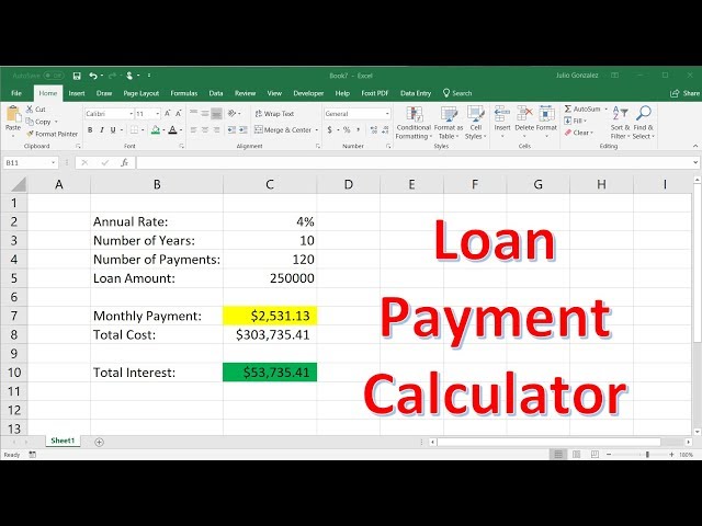
First, we will set up a simple spreadsheet with the information we need to calculate the loan payments. We will need the following information:
-The loan amount
-The interest rate
-The term of the loan (in years)
-The start date of the loan
Once we have this information, we can use Excel’s PMT function to calculate the monthly payments. The PMT function takes the following arguments:
-The interest rate (per period)
-The number of periods
-The present value of the loan (the amount you are borrowing)
-The future value of the loan (the amount you will have paid off at the end of the term)
-A value indicating whether the payment is made at the beginning or end of each period
The Formula
The easiest way to calculate loan payments in Excel is with the PMT function. You can use the PMT function to figure out payment amounts for any type of loan, including auto and mortgage loans.
To use the PMT function, you need to know the interest rate, number of periods (years), and loan amount. For example, if you have a 5% interest rate and you want to calculate payments for a 30-year loan, your number of periods would be 360 (30*12).
Here’s the syntax for the PMT function:
=PMT(interest rate per period, number of periods, loan amount)
For example, if you have a $20,000 loan with a 5% interest rate and you want to know what your monthly payments would be for a term of 60 months, you would use this formula:
=PMT(5%/12,60,-20,000)
The “-” sign in front of the loan amount is important — it tells Excel that you want to make payments on a loan (as opposed to receiving payments).
If you want to see what the total cost of the loan will be (including interest), you can use the PV function. The syntax for PV is:
=PV(interest rate per period, number of periods,-payment amount)
For example, if you want to know the total cost of that $20,000 loan from earlier with monthly payments of $377.42 for 60 months, you would use this formula:
=PV(5%/12),60,-377.42)
The PMT Function
The PMT function is classified as a financial function and is used to calculate the periodic payment for a loan based on constant payments and a constant interest rate. The PMT function syntax has the following arguments:
rate – Required. The interest rate of the loan.
nper – Required. The total number of payments for the loan.
pv – Required. The present value, or principal amount of the loan.
fv – Optional. The future value of the loan after nper payments have been made. If omitted, fv defaults to 0 (zero), indicating that there will be no balloon payment at maturity of the loan’s term.
type – Optional. A number that indicates when payments are due:
0 (zero) or omitted– Payments are due at the end of each period payable period (end-of-month). If type is omitted, it is assumed to be 0 (zero).
1– Payments are due at the beginning of each period in payable period (beginning-of-month).
The PV Function
The PV function in Excel can be used to calculate the present value of a loan. The present value is the amount that you would need to pay today in order to have the loan repaid in full by the end of its term. In order to use the PV function, you will need to know the interest rate, the number of payments, and the amount of each payment.
To use the PV function, enter the following into a cell:
=PV(interest rate, number of payments, payment amount)
For example, if you have a 5% interest rate, and you are making monthly payments of $100 for 36 months, you would enter:
=PV(0.05, 36, 100)
This would give you a present value of $3,139.04.
The NPER Function
The NPER function is used to calculate the number of periods for a loan or investment, using the periodic interest rate and constant payment amounts. For example, you can use NPER to calculate the number of monthly payments for a $12,000 loan at a 4.5% annual interest rate, assuming that payments are made monthly.
In the example shown, the formula used to calculate monthly payments is:
= NPER(D5/12,-D6,-D7)
where D5 contains the annual interest rate (4.5%), D6 contains the number of years for the loan term (15), and D7 contains the loan amount (12000).
The FV Function
The FV function in Excel is a financial function that returns the future value of an investment. The future value is calculated using a fixed interest rate and number of payments. You can use the FV function to calculate the future value of both annuity and non-annuity investments.
The syntax for the FV function is:
FV(rate, nper, pmt, [pv], [type])
Where:
rate – the interest rate per period.
nper – the total number of periods.
pmt – the payment per period.
pv – the present value. This is optional if you want to calculate the future value of an annuity (i.e., a series of equal payments). If you omit this argument, it is assumed to be 0 (zero).
type – the type of payment. This is also optional. The type can be 0 (the default) or 1, where 0 indicates that payments are made at the end of each period and 1 indicates that payments are made at the beginning of each period.
Conclusion
Now that you know how to calculate loan payments in Excel, you can use this information to make better financial decisions. If you’re thinking about taking out a loan, you can use Excel to estimate your payments and compare different loan options. You can also use Excel to track your actual payments and see how they compare to your budget.